API Reference¶

Core¶

class pyamica.AMICA(n_components=None, n_models=1, n_mix=3, max_iter=2000, lrate=0.1, lrate0=0.1, lratefact=0.5, rho0=1.5, minrho=1.0, maxrho=2.0, rholrate=0.05, rholratefact=0.5, do_sphere=True, do_newton=True, newt_start=50, newtrate=1.0, newt_ramp=10, doscaling=True, min_dll=1e-09, min_nd=1e-06, use_grad_norm=True, use_min_dll=True, maxdecs=3, maxincs=5, minlrate=1e-08, invsigmax=100.0, invsigmin=1e-08, writestep=100, verbose=True, dtype=torch.float64, device='cpu', chunk_t=None, compile=False, time_iters=False, checkpoint_every=0, checkpoint_path=None, fix_init=False, do_reject=False, reject_sigma=3.0, num_reject=5, reject_start=1, reject_int=1)[source]¶

Bases: object

Adaptive Mixture ICA estimator (scikit-learn-style interface).

Parameters:

n_components (int or None) – Number of ICA components. Default None (equal to number of channels).
n_models (int) – Number of ICA models fitted simultaneously (M). Default 1.
n_mix (int) – Number of generalised-Gaussian mixture components per source (J). Default 3.
max_iter (int) – Hard ceiling on EM iterations. Default 2000.
lrate (float) – Initial learning rate for the natural-gradient A update. Default 0.1.
lrate0 (float) – Maximum learning rate after the ramp-up phase. Default 0.1.
lratefact (float) – Multiplicative reduction applied to lrate when LL decreases. Default 0.5.
rho0 (float) – Initial GGD shape parameter (1 = Laplacian, 2 = Gaussian). Default 1.5.
minrho (float) – Lower clamp on rho. Default 1.0.
maxrho (float) – Upper clamp on rho. Default 2.0.
rholrate (float) – Step size for rho gradient updates. Default 0.05.
rholratefact (float) – Reduction factor applied to rholrate when LL decreases. Default 0.5.
do_sphere (bool) – PCA-whiten the data before ICA. Default True.
do_newton (bool) – Use the Newton correction for W (see Palmer 2008). Default True.
newt_start (int) – Iteration at which to begin Newton steps. Default 50.
newtrate (float) – Newton learning-rate ceiling. Default 1.0.
newt_ramp (int) – Number of ramp-up iterations before reaching newtrate. Default 10.
doscaling (bool) – Rescale A columns to unit norm after each update. Default True.
min_dll (float) – Stop when the LL improvement is below this for maxincs consecutive iterations. Default 1e-9.
min_nd (float) – Stop when gradient norm falls below this. Default 1e-6.
use_grad_norm (bool) – Enable the gradient-norm stopping criterion. Default True.
use_min_dll (bool) – Enable the LL-improvement stopping criterion. Default True.
maxdecs (int) – Number of consecutive LL decreases before halving lrate. Default 3.
maxincs (int) – Number of consecutive iterations below min_dll before stopping. Default 5.
minlrate (float) – Stop if lrate falls below this value. Default 1e-8.
invsigmax (float) – Upper clamp on the inverse scale parameter sbeta. Default 100.0.
invsigmin (float) – Lower clamp on the inverse scale parameter sbeta. Default 1e-8.
writestep (int) – Print a progress line every this many iterations. Default 100.
verbose (bool) – Print training progress. Default True.
dtype (torch.dtype) – Floating-point type. Default torch.float64 (matches Fortran double precision and is required for numerical agreement with the reference).
device (str or torch.device) – Compute device, e.g. 'cpu', 'cuda', 'mps'. Default 'cpu'.
chunk_t (int or None) – Number of time samples per E-step chunk. Limits peak memory to O(chunk_t * M * n * J) instead of O(T * M * n * J), and improves CPU cache utilisation by keeping intermediates in L3. None (default): auto-selected on CPU (targeting ~32 MB); on GPU the full dataset is processed in one pass (maximum parallelism). Set explicitly on GPU if peak VRAM usage is a concern - each (T, M, n, J) intermediate costs roughly T * M * n * J * 8 bytes, and several are live simultaneously. A value of 8192 is a conservative starting point for laptops. or limited VRAM.
compile (bool) – Apply torch.compile to the E-step and M-step before the EM loop. The first iteration incurs a JIT compilation overhead; subsequent iterations benefit from kernel fusion. Default False.
time_iters (bool) – Record wall time for each EM iteration in iter_times_ (list of floats, seconds). For CUDA, a synchronize() call is inserted so times reflect actual GPU work. Default False.
checkpoint_every (int) – Save a checkpoint every this many iterations. 0 disables checkpointing. Default 0.
checkpoint_path (str or None) – File path for the checkpoint. Required if checkpoint_every > 0. If the file exists at the start of fit(), training resumes from that checkpoint. Default None.
fix_init (bool) – If True, skip parameter initialisation and use whatever values are already stored on the instance. Intended for checkpoint resumption; not normally needed directly. Default False.
do_reject (bool) – Enable per-sample outlier rejection during training. When True, time points whose per-sample log-likelihood falls more than reject_sigma standard deviations below the mean are excluded from the EM parameter updates for the remainder of training. The rejection mask is recomputed up to num_reject times. Disabled by default, matching the Fortran default (do_reject 0). Useful for data with large transient artefacts that have not been removed beforehand.
reject_sigma (float) – Number of standard deviations below the mean log-likelihood used as the rejection threshold. A sample at iteration t is excluded when LL_t < mean(LL) - reject_sigma * std(LL). Default 3.0.
num_reject (int) – Maximum number of rejection events. After this many mask updates the rejection mask is frozen for the rest of training. Default 5.
reject_start (int) – Iteration at which the first rejection event may occur. Default 1.
reject_int (int) – Minimum number of iterations between consecutive rejection events. Default 1 (evaluate every iteration until num_reject events have occurred).

__init__(n_components=None, n_models=1, n_mix=3, max_iter=2000, lrate=0.1, lrate0=0.1, lratefact=0.5, rho0=1.5, minrho=1.0, maxrho=2.0, rholrate=0.05, rholratefact=0.5, do_sphere=True, do_newton=True, newt_start=50, newtrate=1.0, newt_ramp=10, doscaling=True, min_dll=1e-09, min_nd=1e-06, use_grad_norm=True, use_min_dll=True, maxdecs=3, maxincs=5, minlrate=1e-08, invsigmax=100.0, invsigmin=1e-08, writestep=100, verbose=True, dtype=torch.float64, device='cpu', chunk_t=None, compile=False, time_iters=False, checkpoint_every=0, checkpoint_path=None, fix_init=False, do_reject=False, reject_sigma=3.0, num_reject=5, reject_start=1, reject_int=1)[source]¶

Parameters:

n_components (int | None)
n_models (int)
n_mix (int)
max_iter (int)
lrate (float)
lrate0 (float)
lratefact (float)
rho0 (float)
minrho (float)
maxrho (float)
rholrate (float)
rholratefact (float)
do_sphere (bool)
do_newton (bool)
newt_start (int)
newtrate (float)
newt_ramp (int)
doscaling (bool)
min_dll (float)
min_nd (float)
use_grad_norm (bool)
use_min_dll (bool)
maxdecs (int)
maxincs (int)
minlrate (float)
invsigmax (float)
invsigmin (float)
writestep (int)
verbose (bool)
dtype (dtype)
device (str)
chunk_t (int | None)
compile (bool)
time_iters (bool)
checkpoint_every (int)
checkpoint_path (str | None)
fix_init (bool)
do_reject (bool)
reject_sigma (float)
num_reject (int)
reject_start (int)
reject_int (int)

fit(X)[source]¶

Fit AMICA to data X.

Parameters:: X (Tensor, shape (T, n_channels)) – T time points, n_channels sensors.
Return type:: self

transform(X)[source]¶

Apply the learned unmixing to new data.

Parameters:: X (Tensor, shape (T, n_channels))
Returns:: sources – Recovered source signals for each of the M models. For a single-model fit (M=1) you can squeeze dim 1.
Return type:: Tensor, shape (T, M, n_components)

fit_transform(X)[source]¶

Fit the model to X and return transformed sources.

Parameters:: X (Tensor)
Return type:: Tensor

property mixing_matrices: Tensor¶: Mixing matrices A, shape (M, n, n). x ≈ A @ s.

property unmixing_matrices: Tensor¶: Unmixing matrices W = inv(A), shape (M, n, n). s = W @ x.

ll_history()[source]¶

Log-likelihood trace up to the last iteration, shape (n_iter_,).

Return type:: Tensor

nd_history()[source]¶

Gradient-norm trace up to the last iteration, shape (n_iter_,).

Return type:: Tensor

save(path)[source]¶

Save the fitted model with torch.save.

Parameters:: path (str)
Return type:: None

classmethod load(path, device='cpu')[source]¶

Load a model saved with save().

Parameters:

path (str)
device (str)

Return type:

AMICA

Examples using `pyamica.AMICA`¶

Basic AMICA Fit

Outlier Rejection

MNE Wrapper¶

class pyamica.AmicaICA(n_components=None, n_models=1, device='cpu', **amica_kwargs)[source]¶

Bases: object

AMICA ICA fitted to MNE Raw or Epochs data.

Parameters:

n_components (int or None) – Number of ICA components. Default None (equal to the number of selected channels).
n_models (int) – Number of AMICA mixture models (M). 1 = standard ICA. M > 1 learns separate unmixing matrices and source densities per mixture model. Default 1.
device (str) – PyTorch device string: 'cpu', 'cuda', or 'mps'. Default 'cpu'.
**amica_kwargs – Passed verbatim to AMICA, e.g. max_iter, lrate, do_newton, compile, time_iters, chunk_t, do_reject, reject_sigma, num_reject, reject_start, reject_int.

Notes

Data are scaled from Volts (MNE convention) to microvolts before fitting. This improves numerical conditioning of the PCA/sphering step and matches the scale on which AMICA’s default hyperparameters were designed. The MNE ICA object returned by to_mne_ica() operates in Volts so it integrates transparently with the rest of MNE.

__init__(n_components=None, n_models=1, device='cpu', **amica_kwargs)[source]¶

Parameters:

n_components (int | None)
n_models (int)
device (str)

fit(inst, picks='eeg')[source]¶

Fit AMICA on the good data in inst.

Bad channels (inst.info['bads']) and bad time segments (BAD annotations in Raw; rejected Epochs) are automatically excluded via MNE’s built-in data extraction.

Parameters:

inst (mne.io.BaseRaw or mne.BaseEpochs)
picks (str or list of str) – Channel type string (‘eeg’, ‘meg’, ‘grad’, ‘mag’) or explicit list of channel names.

Return type:

self

plot_model_posteriors(ax=None, figsize=None)[source]¶

Plot per-time-point model posteriors p(m|t) against recording time.

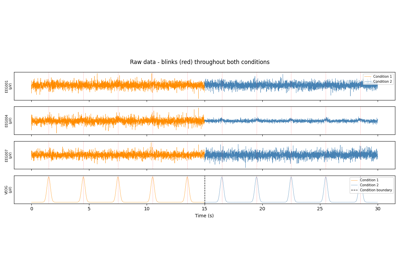
Each line shows the probability that model m is active at each sample. For well-separated conditions the lines should approach 0/1 in distinct time segments, making it easy to verify that AMICA’s learned models align with the known experimental conditions.

Parameters:

ax (matplotlib.axes.Axes or None) – Axes to plot into. If None, a new figure is created.
figsize (tuple or None) – Figure size passed to plt.figure(). Ignored if ax is given.

Return type:

matplotlib.axes.Axes

plot_model_dominance(smooth_s=0.0, figsize=None, ax=None)[source]¶

Stacked area chart of model posteriors, easier to read than overlapping lines when models switch rapidly.

Because posteriors sum to 1, each model’s share is shown as a filled band. Rapid within-second switches appear as mixed colours rather than unreadable flickering.

An optional Gaussian smooth (smooth_s seconds) can be applied before plotting to suppress fast transients and reveal the broader structure of model dominance.

Parameters:

smooth_s (float) – Standard deviation of the Gaussian kernel (seconds). 0 (default) means no smoothing.
ax (matplotlib.axes.Axes or None) – Axes to plot into. If None, a new figure is created.
figsize (tuple or None) – Figure size. Ignored when ax is given.

Return type:

matplotlib.axes.Axes

get_mne_ica(model_idx=0)[source]¶

Return the cached mne.preprocessing.ICA for model_idx.

The object is created on first access and cached; subsequent calls return the same object so that interactive exclusion selections (ica.exclude) made in plot_sources / plot_components are preserved and picked up by apply().

Parameters:: model_idx (int) – 0-indexed model. Model 0 is always the most probable model after fit().

plot_sources(inst, model_idx=0, **kwargs)[source]¶

Plot ICA source time-courses for model_idx (delegates to MNE).

Clicking on a source in the interactive window marks it for removal; selections are stored on the cached MNE ICA object and read by apply().

Parameters:

inst (mne.io.BaseRaw or mne.BaseEpochs)
model_idx (int) – Which AMICA model to inspect. Default 0.
**kwargs – Forwarded to mne.preprocessing.ICA.plot_sources().

plot_components(inst=None, model_idx=0, **kwargs)[source]¶

Plot ICA component topographies for model_idx (delegates to MNE).

Parameters:

inst (mne.io.BaseRaw or mne.BaseEpochs or None)
model_idx (int) – Which AMICA model to inspect. Default 0.
**kwargs – Forwarded to mne.preprocessing.ICA.plot_components().

plot_properties(inst, picks=None, model_idx=0, **kwargs)[source]¶

Plot detailed component properties for model_idx (delegates to MNE).

Parameters:

inst (mne.io.BaseRaw or mne.BaseEpochs)
picks (int or list of int or None) – Component indices to plot. None = all.
model_idx (int) – Which AMICA model to inspect. Default 0.
**kwargs – Forwarded to mne.preprocessing.ICA.plot_properties().

plot_overlay(inst, model_idx=0, **kwargs)[source]¶

Plot original vs. ICA-cleaned signal for model_idx (delegates to MNE).

Uses the excluded components stored on the cached MNE ICA object, so call this after marking components via plot_sources() to preview what will be removed.

Parameters:

inst (mne.io.BaseRaw or mne.Evoked)
model_idx (int) – Which AMICA model to inspect. Default 0.
**kwargs – Forwarded to mne.preprocessing.ICA.plot_overlay().

plot_scores(scores, model_idx=0, **kwargs)[source]¶

Plot component scores (e.g. from find_bads_eog) for model_idx.

Typical usage:

eog_idx, scores = ica.find_bads_eog(raw, model_idx=m, ch_name='HEOG')
ica.plot_scores(scores, model_idx=m)

Parameters:

scores (array-like) – Scores returned by find_bads_eog() or find_bads_ecg().
model_idx (int) – Which AMICA model the scores belong to. Default 0.
**kwargs – Forwarded to mne.preprocessing.ICA.plot_scores().

find_bads_eog(inst, model_idx=0, **kwargs)[source]¶

Identify EOG-correlated components for model_idx (delegates to MNE).

Parameters:

inst (mne.io.BaseRaw or mne.BaseEpochs)
model_idx (int) – Which AMICA model to inspect. Default 0.
**kwargs – Forwarded to mne.preprocessing.ICA.find_bads_eog() (e.g. ch_name, threshold, measure).

Returns:

eog_indices (list of int)
scores (ndarray)

find_bads_ecg(inst, model_idx=0, **kwargs)[source]¶

Identify ECG-correlated components for model_idx (delegates to MNE).

Parameters:

inst (mne.io.BaseRaw or mne.BaseEpochs)
model_idx (int) – Which AMICA model to inspect. Default 0.
**kwargs – Forwarded to mne.preprocessing.ICA.find_bads_ecg() (e.g. ch_name, threshold, method).

Returns:

ecg_indices (list of int)
scores (ndarray)

review(inst, model_idx=0, eog_ch=None, ecg_ch=None, eog_kwargs=None, ecg_kwargs=None)[source]¶

Semi-automatic component review for one model.

Runs automated bad-component detection, prints a terminal summary, pre-selects flagged components, then opens plot_sources() so you can confirm or adjust the selection interactively before closing the window.

Parameters:

inst (mne.io.BaseRaw or mne.BaseEpochs)
model_idx (int) – Which AMICA model to review. Default 0.
eog_ch (str or list of str or None) – EOG channel name(s) to pass to find_bads_eog(). Pass a list to run detection separately for each channel (e.g. ['HEOG', 'VEOG']).
ecg_ch (str or None) – ECG channel name for find_bads_ecg().
eog_kwargs (dict or None) – Extra keyword arguments for find_bads_eog().
ecg_kwargs (dict or None) – Extra keyword arguments for find_bads_ecg().

Returns:

Final component exclusion list for this model (same object as get_mne_ica(model_idx).exclude).

Return type:

list of int

Example

for m in range(ica.n_models):
    ica.review(raw, model_idx=m,
               eog_ch=['HEOG', 'VEOG'], ecg_ch='ECG')
ica.apply(raw)

score_dipolarity(inst, model_idx=0)[source]¶

Score each IC by how well its topomap resembles a single dipole.

A dipolar scalp field varies roughly linearly across the electrode array. This method fits a linear regression of each IC topomap onto the x/y channel coordinates and returns the coefficient of determination (R squared). Values close to 1 indicate a dipolar pattern; values near 0 indicate a spatially diffuse or noisy map.

This is a fast proxy for dipolarity: a linear fit on x/y channel positions captures the dominant spatial gradient of a single dipole without requiring a full head model.

Parameters:

inst (mne.io.BaseRaw or mne.BaseEpochs or mne.Evoked) – Used only for channel position information. Channels with missing or invalid positions (zero norm or NaN, which MNE assigns when no montage is set) are silently excluded from the regression. An error is only raised when no valid positions remain at all.
model_idx (int) – Which AMICA model to score. Default 0.

Returns:

scores – R squared of the linear fit for each IC topomap. Higher values indicate more dipolar patterns.

Return type:

np.ndarray, shape (n_components,)

Raises:

RuntimeError – If fit() has not been called yet.
ValueError – If no EEG channels with valid positions are found. This happens when no montage has been applied, since MNE initialises all channel locations to zero by default. Apply a montage first, e.g. inst.set_montage('standard_1020').

score_mutual_information(inst, model_idx=0, n_bins=30)[source]¶

Compute the pairwise mutual information matrix between IC time series.

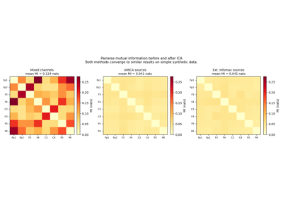
Mutual information (MI) measures statistical dependence between two signals: zero means complete independence, larger values indicate stronger dependence. ICA aims to minimise MI between components, so a well-fitted decomposition should produce a matrix that is close to zero everywhere off the diagonal.

MI is estimated from a joint histogram with n_bins per dimension. The estimator is biased towards zero for small T; use at least T = 1000 samples for reliable values.

Parameters:

inst (mne.io.BaseRaw or mne.BaseEpochs) – Data to extract IC time series from.
model_idx (int) – Which AMICA model to score. Default 0.
n_bins (int) – Number of histogram bins per dimension. Default 30.

Returns:

mi – Symmetric matrix of pairwise MI values in nats. Diagonal is zero.

Return type:

np.ndarray, shape (n_components, n_components)

Raises:

RuntimeError – If fit() has not been called yet.

apply(inst)[source]¶

Apply ICA artifact removal in-place.

Component exclusions are read from the cached MNE ICA objects. Set them interactively via plot_sources() / plot_components(), or directly via get_mne_ica(m).exclude = [0, 2].

For n_models=1 this delegates directly to MNE’s ICA.apply(). For n_models>1 a hard per-sample model assignment (argmax of posteriors) selects which model’s unmixing and exclusion list is used at each time point.

Parameters:: inst (mne.io.BaseRaw or mne.BaseEpochs) – Modified in-place.
Return type:: inst

save(path)[source]¶

Save the fitted model and component selections to a .amica file.

The file is a compressed NumPy archive containing all fitted tensors, recording metadata, and per-model exclusion lists. Reload with AmicaICA.load(path).

Parameters:: path (str or Path) – Output path. .amica.npz is appended if not already present.
Return type:: None

classmethod load(path)[source]¶

Load a fitted AmicaICA from a .amica file saved with save().

All fitted tensors and per-model exclusion lists are restored. Call apply(inst) afterwards to clean the original recording.

Parameters:: path (str or Path) – Path to the .amica.npz file.
Return type:: AmicaICA

to_mne_ica(model_idx=0)[source]¶

Build and return a fitted mne.preprocessing.ICA object.

After fit(), AMICA models are sorted so that model 0 is always the most probable model (highest gm_) and components within each model are ordered by decreasing variance explained. For multi-model fits, call once per model:

ica0 = amica_ica.to_mne_ica(model_idx=0) # most probable model ica1 = amica_ica.to_mne_ica(model_idx=1)

AMICA’s ZCA sphere and W matrix are decomposed into MNE’s internal PCA + ICA representation:

pca_components_ = V.T (orthonormal PCA eigenvectors)
unmixing_matrix_ = W × V × diag(D⁻½)
mixing_matrix_ = diag(D^½) × V.T × A

where V, D come from the ZCA sphere (shared across all models) and A = inv(W) is AMICA’s mixing matrix for the selected model.

Parameters:: model_idx (int) – Which AMICA model to export (0-indexed). Default 0 (most probable model after fit()).
Returns:: Fully populated, ready for plot_components(), find_bads_eog(), apply(), save() / load().
Return type:: mne.preprocessing.ICA

Examples using `pyamica.AmicaICA`¶

Artefact Removal with Multi-Model AMICA

MNE-Python Workflow

Mutual Information Reduction

API Reference¶

Core¶

Examples using pyamica.AMICA¶

MNE Wrapper¶

Examples using pyamica.AmicaICA¶

Examples using `pyamica.AMICA`¶

Examples using `pyamica.AmicaICA`¶