Artefact Removal with Multi-Model AMICA

Demonstrates the full artefact-removal workflow on data with two distinct experimental conditions and blink artefacts occurring throughout both.

With M=2 AMICA each model gets its own ICA decomposition, so the blink component is identified separately per model. When applying, apply() uses the dominant model’s decomposition at each time point - artefact removal is always done with the most appropriate model. This is something single-model ICA cannot do.

import numpy as np
import mne
import matplotlib.pyplot as plt

from pyamica import AmicaICA

mne.set_log_level("WARNING")

Synthetic Two-Condition EEG with Blinks

Two 15-second conditions with different scalp mixing matrices - mimicking two experimental conditions with different functional connectivity (e.g. eyes-open vs eyes-closed, fixation vs free-viewing). Both conditions have Laplacian-distributed sources. Blinks (~25 µV) occur throughout both.

Blink construction: the blink topography is the 8th column of both A1 and A2. After ICA, the blink maps onto exactly one IC per model, making find_bads_eog() trivially reliable.

rng   = np.random.default_rng(42)
sfreq = 250
n_eeg = 8
n_src = n_eeg - 1    # 7 brain sources; 8th direction reserved for blink
half  = sfreq * 15   # 15 s per condition
T     = 2 * half     # 30 s total

# Shared blink column → same independent direction in both mixing matrices
blink_col = rng.standard_normal(n_eeg)

# Two different mixing matrices (different scalp projections, same blink column)
B1 = rng.standard_normal((n_eeg, n_src))
B2 = rng.standard_normal((n_eeg, n_src))
A1 = np.column_stack([B1, blink_col])   # condition-1 mixing matrix
A2 = np.column_stack([B2, blink_col])   # condition-2 mixing matrix

# Brain sources: Laplacian in both conditions (same statistics, different realisation)
src1 = rng.laplace(0, 1, (n_src, half)) * 1e-5
src2 = rng.laplace(0, 1, (n_src, half)) * 1e-5

brain = np.concatenate([B1 @ src1, B2 @ src2], axis=1)   # (n_eeg, T)

# Blink signal in the shared column direction
blink_times = np.arange(1.5, 30.0, 3.0)
t_arr = np.arange(T) / sfreq
blink = sum(
    np.exp(-0.5 * ((t_arr - bt) / 0.15) ** 2)
    for bt in blink_times
) * 25e-6

eeg_data  = brain + blink_col[:, None] * blink[None, :]
veog_data = blink[None, :]

data = np.vstack([eeg_data, veog_data])
ch_names = [f"EEG{i:03d}" for i in range(1, n_eeg + 1)] + ["VEOG"]
ch_types = ["eeg"] * n_eeg + ["eog"]

info = mne.create_info(ch_names=ch_names, sfreq=sfreq, ch_types=ch_types)
raw  = mne.io.RawArray(data, info, verbose=False)

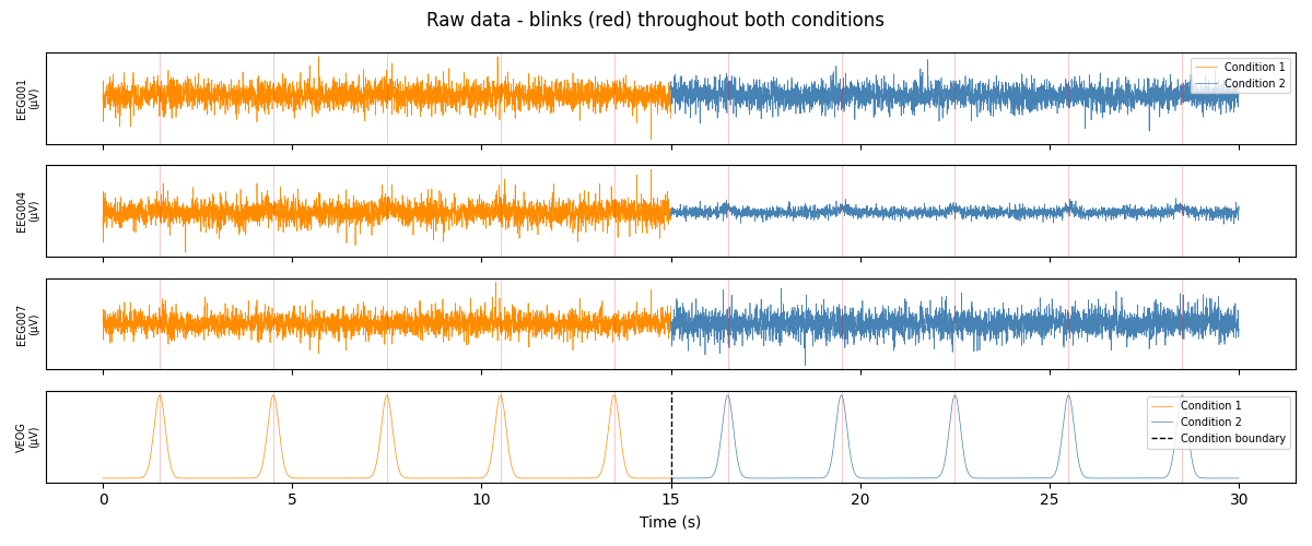
Raw Data

Both conditions share the same amplitude distribution (Laplacian), but their inter-channel correlations differ because A1 ≠ A2. Blinks (red lines) appear throughout both halves.

fig, axes = plt.subplots(4, 1, figsize=(12, 5), sharex=True)
for ax, ch_idx in zip(axes, [0, 3, 6, n_eeg]):
    ax.plot(raw.times[:half], data[ch_idx, :half] * 1e6,
            lw=0.5, color="darkorange", label="Condition 1")
    ax.plot(raw.times[half:], data[ch_idx, half:] * 1e6,
            lw=0.5, color="steelblue", label="Condition 2")
    for bt in blink_times:
        ax.axvline(bt, color="red", lw=0.4, alpha=0.4)
    ax.set_ylabel(f"{ch_names[ch_idx]}\n(µV)", fontsize=7)
    ax.set_yticks([])
axes[0].legend(loc="upper right", fontsize=7)
axes[-1].axvline(15.0, color="k", linestyle="--", lw=1.0, label="Condition boundary")
axes[-1].legend(loc="upper right", fontsize=7)
axes[-1].set_xlabel("Time (s)")
fig.suptitle("Raw data - blinks (red) throughout both conditions")
fig.tight_layout()
plt.show()

Fit AmicaICA M=2

AMICA discovers the two mixing matrices and fits a separate ICA decomposition for each condition. Because the source statistics are identical, model assignment is driven purely by spatial structure (which W best demixes the data at each time point). Blink samples contribute equal likelihood to both models and do not bias the assignments.

import torch; torch.manual_seed(0)

ica = AmicaICA(n_models=2, max_iter=200, verbose=False)
ica.fit(raw, picks="eeg")

gm = ica._model.gm_.numpy()
print(f"Global model weights: {gm.round(3)}")

Global model weights: [0.5 0.5]

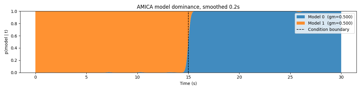
Model Dominance

The two models split cleanly at 15 s. Unlike uniform-vs-Laplacian data, blink peaks do not bleed into the wrong model because both models carry the same Laplacian prior; blink samples look equally plausible under either.

ax = ica.plot_model_dominance(smooth_s=0.2, figsize=(12, 3))
ax.axvline(15.0, color="k", linestyle="--", lw=1.2, label="Condition boundary")
ax.legend(loc="upper right")
plt.show()

The review() Workflow

In practice, review each model interactively:

for m in range(ica.n_models):
    ica.review(raw, model_idx=m, eog_ch="VEOG")
ica.apply(raw)

review() runs automated EOG/ECG detection, pre-selects flagged components, then opens plot_sources() for interactive confirmation. Each model is reviewed independently - the blink component may land on a different IC index in each condition’s decomposition.

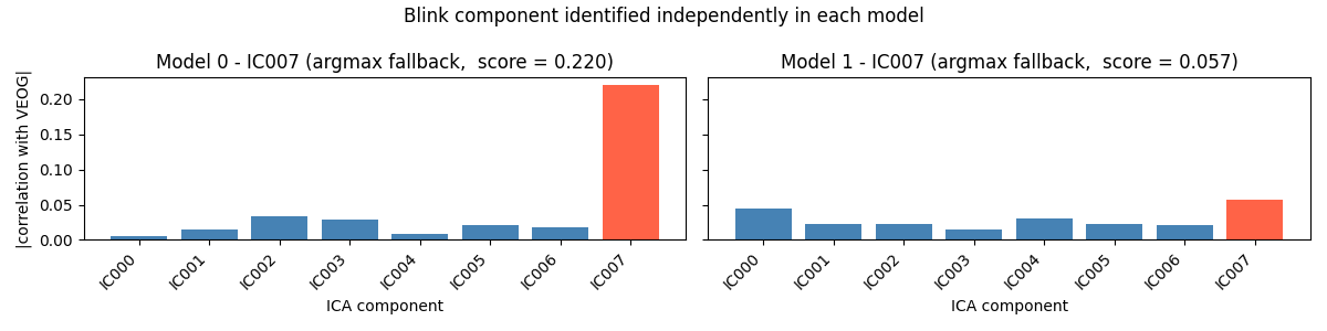
Identify Blink Component per Model

Because the blink occupies the 8th independent direction of both A1 and A2, one IC per model has near-perfect VEOG correlation. find_bads_eog() detects it automatically. Using measure='correlation' with a moderate threshold rather than the default z-score, which can be too conservative when the number of components is small (n=8).

fig, axes = plt.subplots(1, 2, figsize=(12, 3), sharey=True)
for m, ax in enumerate(axes):
    eog_idx, scores = ica.find_bads_eog(
        raw, model_idx=m, ch_name="VEOG",
        measure="correlation", threshold=0.5,
    )
    comp = eog_idx[0] if eog_idx else int(np.argmax(np.abs(scores)))
    colors = ["tomato" if i == comp else "steelblue" for i in range(n_eeg)]
    ax.bar(range(n_eeg), np.abs(scores), color=colors)
    tag = "auto-detected" if eog_idx else "argmax fallback"
    ax.set_title(f"Model {m} - IC{comp:03d} ({tag},  score = {np.abs(scores[comp]):.3f})")
    ax.set_xlabel("ICA component")
    ax.set_xticks(range(n_eeg))
    ax.set_xticklabels([f"IC{i:03d}" for i in range(n_eeg)], rotation=45, ha="right")
axes[0].set_ylabel("|correlation with VEOG|")
fig.suptitle("Blink component identified independently in each model")
fig.tight_layout()
plt.show()

Set Per-Model Exclusions and Apply

Exclude the blink component from each model independently, then apply. apply() uses per-sample posterior assignment to decide which model’s exclusion list to use at each time point.

for m in range(ica.n_models):
    eog_idx, scores = ica.find_bads_eog(
        raw, model_idx=m, ch_name="VEOG",
        measure="correlation", threshold=0.5,
    )
    if not eog_idx:
        eog_idx = [int(np.argmax(np.abs(scores)))]
    ica.get_mne_ica(m).exclude = eog_idx
    print(f"Model {m}: excluding IC{eog_idx[0]:03d}")

raw_clean = raw.copy()
ica.apply(raw_clean)

Model 0: excluding IC007
Model 1: excluding IC007

	General
	MNE object type	RawArray
	Measurement date	Unknown
	Participant	Unknown
	Experimenter	Unknown
	Acquisition
	Duration	00:00:30 (HH:MM:SS)
	Sampling frequency	250.00 Hz
	Time points	7,500
	Channels
	EEG	8
	EOG	1
	Head & sensor digitization	Not available
	Filters
	Highpass	0.00 Hz
	Lowpass	125.00 Hz

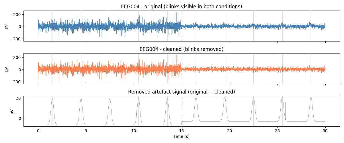
Before and After

EEG001 (most blink-contaminated channel in this realisation) before and after removal. Blinks are suppressed in both conditions.

fig, axes = plt.subplots(3, 1, figsize=(12, 5), sharex=True)
orig_µV  = raw.get_data(picks="eeg")[3] * 1e6
clean_µV = raw_clean.get_data(picks="eeg")[3] * 1e6

axes[0].plot(raw.times, orig_µV,  lw=0.5, color="steelblue")
axes[0].set_title("EEG004 - original (blinks visible in both conditions)")
axes[0].set_ylabel("µV")

axes[1].plot(raw.times, clean_µV, lw=0.5, color="coral")
axes[1].set_title("EEG004 - cleaned (blinks removed)")
axes[1].set_ylabel("µV")

axes[2].plot(raw.times, orig_µV - clean_µV, lw=0.5, color="gray")
axes[2].set_title("Removed artefact signal (original − cleaned)")
axes[2].set_ylabel("µV")
axes[2].set_xlabel("Time (s)")

for ax in axes:
    ax.axvline(15.0, color="k", linestyle="--", lw=0.8)
    for bt in blink_times:
        ax.axvline(bt, color="red", lw=0.4, alpha=0.3)

fig.tight_layout()
plt.show()

removed_peak   = np.abs(orig_µV - clean_µV).max()
remaining_peak = np.abs(clean_µV).max()
print(f"Removed signal peak:   {removed_peak:.1f} µV")
print(f"Remaining signal peak: {remaining_peak:.1f} µV")

Removed signal peak:   20.7 µV
Remaining signal peak: 244.9 µV