Outlier Rejection

Demonstrates the do_reject feature on heavily contaminated synthetic data. AMICA identifies and excludes time points whose per-sample log-likelihood falls more than reject_sigma standard deviations below the mean, then immediately re-runs the E-step so the M-step already uses clean statistics. Up to num_reject rejection events are allowed; after that the mask is frozen.

The contamination here is 120 spike transients at 15x the signal standard deviation in a 2000-sample recording (6 percent of samples contaminated). This is severe enough that standard ICA is noticeably biased, while AMICA with rejection recovers the true mixing matrix accurately.

import numpy as np
import torch
import matplotlib.pyplot as plt
from scipy.optimize import linear_sum_assignment

from pyamica import AMICA

torch.manual_seed(0)
rng = np.random.default_rng(42)

Synthetic Data with Heavy Contamination

Eight independent Laplacian sources mixed by a random matrix. Columns of A_true are unit-normalised so channel variance is ~1. 120 spike transients at 15x amplitude are inserted at random positions, contaminating about 6 percent of all samples.

n_ch, T  = 8, 2000
n_spikes = 120
amp      = 15.0

sources = rng.laplace(0, 1, (n_ch, T))
A_true  = rng.standard_normal((n_ch, n_ch))
A_true /= np.linalg.norm(A_true, axis=0, keepdims=True)

clean        = (A_true @ sources).T.astype("float64")   # (T, n_ch)
spike_idx    = np.sort(rng.choice(T, size=n_spikes, replace=False))
contaminated = clean.copy()
contaminated[spike_idx] *= amp

X = torch.from_numpy(contaminated)

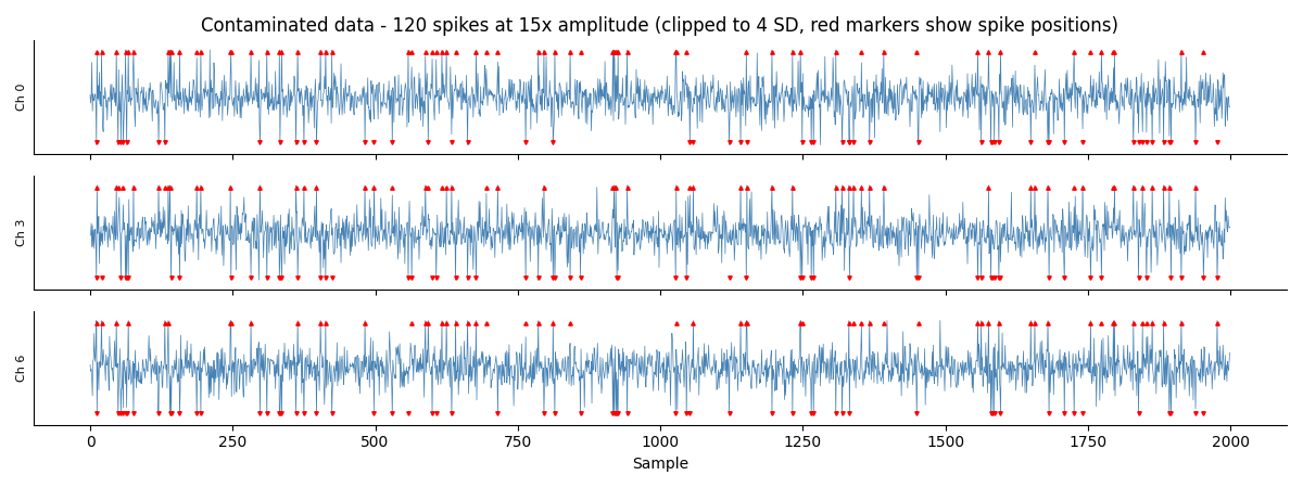
Raw Data

Y-axis clipped to 4 standard deviations of the clean signal. At 15x amplitude the spikes go far off-screen; their positions are marked with red tick marks at the clip boundary.

t       = np.arange(T)
sigma   = clean.std(axis=0)
ch_plot = [0, 3, 6]

fig, axes = plt.subplots(len(ch_plot), 1, figsize=(12, 4.5), sharex=True)
for ax, ch in zip(axes, ch_plot):
    clip = 4.0 * sigma[ch]
    ax.plot(t, contaminated[:, ch].clip(-clip, clip), lw=0.5, color="steelblue")
    for s in spike_idx:
        sign = np.sign(contaminated[s, ch]) or 1
        ax.plot(s, sign * clip * 0.95, marker="v" if sign < 0 else "^",
                color="red", ms=2.5, zorder=3)
    ax.set_ylim(-clip * 1.2, clip * 1.2)
    ax.set_ylabel(f"Ch {ch}", fontsize=8)
    ax.set_yticks([])
    ax.spines[["top", "right"]].set_visible(False)
axes[-1].set_xlabel("Sample")
axes[0].set_title(
    f"Contaminated data - {n_spikes} spikes at {amp:.0f}x amplitude "
    f"(clipped to 4 SD, red markers show spike positions)")
fig.tight_layout()
plt.show()

Fit Without and With Rejection

model_plain = AMICA(n_models=1, max_iter=200, verbose=False)
model_plain.fit(X)

model_rej = AMICA(n_models=1, max_iter=200, verbose=False,
                  do_reject=True, reject_sigma=3.0,
                  num_reject=5, reject_start=10, reject_int=10)
model_rej.fit(X)

mask_np    = model_rej._rej_mask_.cpu().numpy()
n_rejected = int((~mask_np).sum())
print(f"Without rejection:  final LL = {model_plain.ll_history()[-1]:.4f}")
print(f"With rejection:     final LL = {model_rej.ll_history()[-1]:.4f}  "
      f"({n_rejected}/{T} samples excluded, {n_spikes} true spikes)")

Without rejection:  final LL = -1.8055
With rejection:     final LL = -1.5096  (96/2000 samples excluded, 120 true spikes)

Rejection Mask Overlaid on Raw Data

The same channel as the top row above, now with rejected time points shaded in red. The mask correctly captures the spike positions.

fig, axes = plt.subplots(2, 1, figsize=(12, 3.5), sharex=True,
                         gridspec_kw={"height_ratios": [3, 1]})

ax_sig, ax_mask = axes
clip = 4.0 * sigma[0]

ax_sig.plot(t, contaminated[:, 0].clip(-clip, clip),
            lw=0.5, color="steelblue", zorder=2)
rejected_t = np.where(~mask_np)[0]
for s in rejected_t:
    ax_sig.axvspan(s - 0.5, s + 0.5, color="tomato", alpha=0.5, zorder=1)
ax_sig.set_ylim(-clip * 1.15, clip * 1.15)
ax_sig.set_ylabel("Ch 0", fontsize=8)
ax_sig.set_yticks([])
ax_sig.spines[["top", "right"]].set_visible(False)
ax_sig.set_title("Rejection mask overlaid on raw data (red = excluded)")

ax_mask.fill_between(t, (~mask_np).astype(float),
                     color="tomato", alpha=0.8, step="mid")
ax_mask.fill_between(t, mask_np.astype(float),
                     color="steelblue", alpha=0.3, step="mid")
ax_mask.set_yticks([0.5])
ax_mask.set_yticklabels(["rejected"], fontsize=7)
ax_mask.set_ylim(0, 1)
ax_mask.set_xlabel("Sample")
ax_mask.spines[["top", "right"]].set_visible(False)

fig.tight_layout()
plt.show()

n_correct  = int(np.isin(rejected_t, spike_idx).sum())
n_false    = n_rejected - n_correct
n_missed   = n_spikes - n_correct
print(f"Correctly rejected (true spikes): {n_correct}/{n_spikes}")
print(f"False rejections (clean samples): {n_false}")
print(f"Missed spikes:                    {n_missed}")

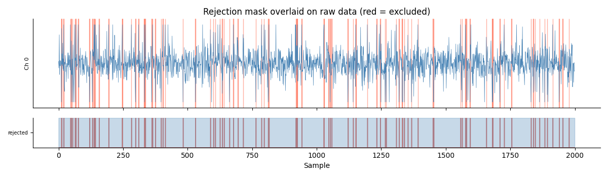
Correctly rejected (true spikes): 96/120
False rejections (clean samples): 0
Missed spikes:                    24

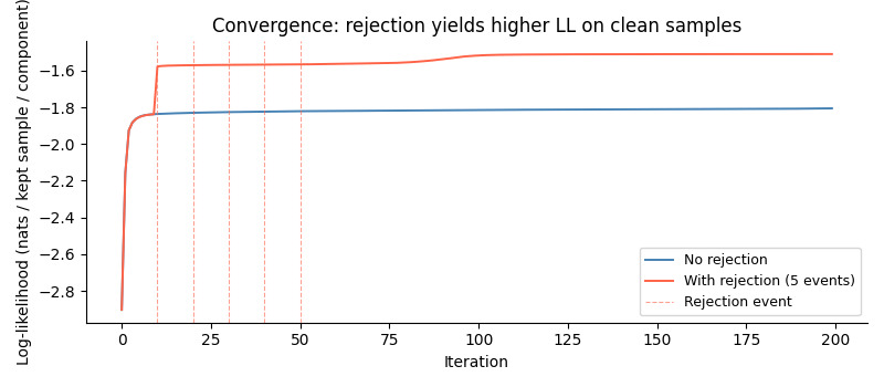
Log-Likelihood Convergence

Both LL curves are per-kept-sample, so they are directly comparable. Without rejection the model spends capacity fitting the spike distribution and converges to a lower LL.

ll_plain = model_plain.ll_history().numpy()
ll_rej   = model_rej.ll_history().numpy()

reject_iters = range(
    model_rej.reject_start,
    model_rej.reject_start + model_rej.num_reject * model_rej.reject_int,
    model_rej.reject_int,
)

fig, ax = plt.subplots(figsize=(8, 3.5))
ax.plot(ll_plain, color="steelblue", lw=1.4, label="No rejection")
ax.plot(ll_rej,   color="tomato",    lw=1.4, label="With rejection (5 events)")
for i, it in enumerate(reject_iters):
    ax.axvline(it, color="tomato", lw=0.8, linestyle="--", alpha=0.6,
               label="Rejection event" if i == 0 else None)
ax.set_xlabel("Iteration")
ax.set_ylabel("Log-likelihood (nats / kept sample / component)")
ax.set_title("Convergence: rejection yields higher LL on clean samples")
ax.legend(fontsize=9)
ax.spines[["top", "right"]].set_visible(False)
fig.tight_layout()
plt.show()

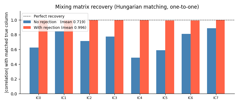
Mixing Matrix Recovery

The estimated A is projected back to sensor space and matched to the true columns using the Hungarian algorithm (optimal one-to-one assignment). A correlation of 1.0 means perfect recovery of that source.

def _hungarian_corr(A_est, A_ref):
    """Optimal one-to-one column matching by absolute correlation."""
    A_en = A_est / (np.linalg.norm(A_est, axis=0, keepdims=True) + 1e-30)
    A_rn = A_ref / (np.linalg.norm(A_ref, axis=0, keepdims=True) + 1e-30)
    C    = np.abs(A_en.T @ A_rn)                   # (n, n)
    row, col = linear_sum_assignment(-C)            # maximise total correlation
    return C[row, col]                              # (n,) matched correlations

S            = model_plain.sphere_.cpu().numpy()
A_plain_full = np.linalg.pinv(S) @ model_plain.A_[0].cpu().numpy()
A_rej_full   = np.linalg.pinv(S) @ model_rej.A_[0].cpu().numpy()

corr_plain = _hungarian_corr(A_plain_full, A_true)
corr_rej   = _hungarian_corr(A_rej_full,   A_true)

x     = np.arange(n_ch)
width = 0.35
fig, ax = plt.subplots(figsize=(8, 3.5))
ax.bar(x - width / 2, corr_plain, width, color="steelblue",
       label=f"No rejection   (mean {corr_plain.mean():.3f})")
ax.bar(x + width / 2, corr_rej,   width, color="tomato",
       label=f"With rejection (mean {corr_rej.mean():.3f})")
ax.axhline(1.0, color="k", lw=0.8, linestyle="--", label="Perfect recovery")
ax.set_xticks(x)
ax.set_xticklabels([f"IC{i}" for i in range(n_ch)], fontsize=8)
ax.set_ylabel("|correlation| with matched true column")
ax.set_ylim(0, 1.12)
ax.set_title("Mixing matrix recovery (Hungarian matching, one-to-one)")
ax.legend(fontsize=9)
ax.spines[["top", "right"]].set_visible(False)
fig.tight_layout()
plt.show()