MNE-Python Workflow

Fit AmicaICA on synthetic EEG data with two mixture models, verify that AMICA correctly assigns each data segment to the right model, and confirm that reconstructing the signal without exclusions is a perfect round-trip.

Note

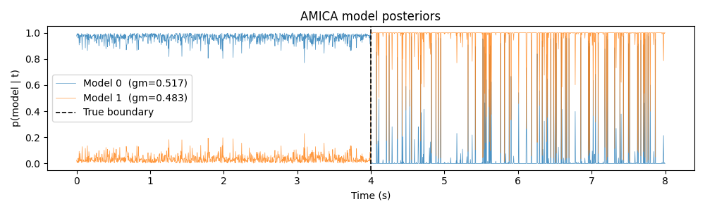
Why are there occasional jumps in the Laplacian segment?

A Laplacian distribution peaks at zero - so when sources produce near-zero values the evidence is equally consistent with the uniform model. AMICA’s posteriors reflect genuine uncertainty at those samples. Soft assignment is correct Bayesian behaviour, not a bug.

The data is constructed entirely from random numbers - no external dataset is required.

import numpy as np
import mne
import matplotlib.pyplot as plt

from pyamica import AmicaICA

mne.set_log_level("WARNING")

Synthetic Two-Segment Raw

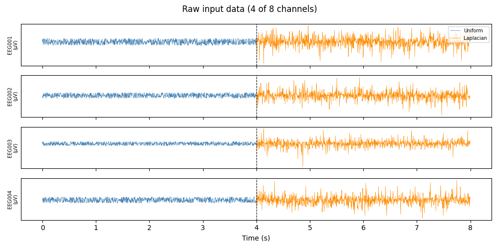
8 EEG channels, 250 Hz, 8 seconds. First 4 s: spatially uniform activity, bounded and sub-Gaussian (std ≈ 5.8 µV). Last 4 s: Laplacian activity, heavy-tailed and super-Gaussian (std ≈ 14 µV).

The distributions are deliberately kept at different scales so their statistical character is visually and numerically distinct.

rng   = np.random.default_rng(42)
sfreq = 250
n_ch  = 8
T     = sfreq * 8   # 8 s
q     = T // 2

ch_names = [f"EEG{i:03d}" for i in range(1, n_ch + 1)]
info = mne.create_info(ch_names=ch_names, sfreq=sfreq, ch_types="eeg")

data = np.concatenate([
    rng.uniform(-1, 1, (n_ch, q)) * 1e-5,  # uniform: bounded in [-1e-5, 1e-5]
    rng.laplace(0, 1,  (n_ch, q)) * 1e-5,  # Laplacian: heavy tails beyond ±1e-5
], axis=1)

raw = mne.io.RawArray(data, info, verbose=False)

Raw Data

The two data segments are clearly visible: the first half has a hard amplitude ceiling (uniform), while the second half has occasional large spikes (Laplacian). The spiky samples near zero in the Laplacian segment are the ones that cause the posterior jumps explained above.

times = raw.times
fig, axes = plt.subplots(4, 1, figsize=(10, 5), sharex=True)
for i, ax in enumerate(axes):
    ax.plot(times[:q], data[i, :q] * 1e6, lw=0.5, color="steelblue",
            label="Uniform")
    ax.plot(times[q:], data[i, q:] * 1e6, lw=0.5, color="darkorange",
            label="Laplacian")
    ax.axvline(4.0, color="k", linestyle="--", lw=0.8)
    ax.set_ylabel(f"{ch_names[i]}\n(µV)", fontsize=7)
    ax.set_yticks([])
axes[0].legend(loc="upper right", fontsize=7)
axes[-1].set_xlabel("Time (s)")
fig.suptitle("Raw input data (4 of 8 channels)")
fig.tight_layout()
plt.show()

Fit AmicaICA (M=2)

ica = AmicaICA(n_models=2, max_iter=200, verbose=False)
ica.fit(raw, picks="eeg")

print(f"Fitted {ica._model.n_iter_} iterations")
print(f"Global model weights: {ica._model.gm_.numpy().round(3)}")

Fitted 200 iterations
Global model weights: [0.517 0.483]

Model Posteriors

Raw per-sample posteriors p(model | t). The transition at 4 s and the occasional ambiguous samples in the Laplacian half are both visible.

ax = ica.plot_model_posteriors(figsize=(10, 3))
ax.axvline(4.0, color="k", linestyle="--", lw=1.2, label="True boundary")
ax.legend()
plt.show()

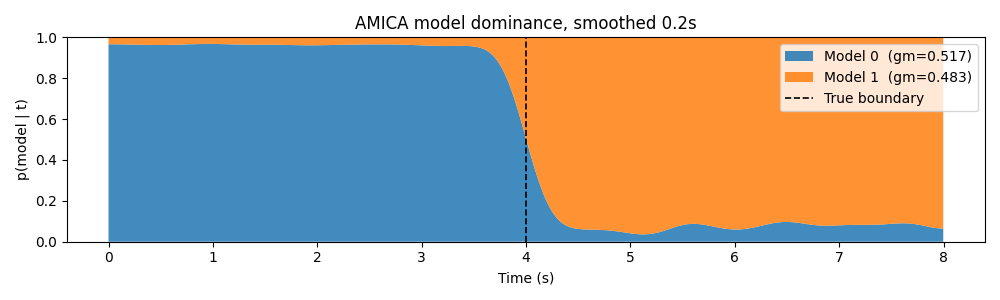
Model Dominance (Stacked Area)

Gaussian smoothing (0.2 s) suppresses per-sample noise while preserving the coarse structure. Ambiguous samples appear as mixed-colour bands.

ax = ica.plot_model_dominance(smooth_s=0.2, figsize=(10, 3))
ax.axvline(4.0, color="k", linestyle="--", lw=1.2, label="True boundary")
ax.legend(loc="upper right")
plt.show()

Separation Accuracy

post     = ica._model.posteriors_.numpy()   # (2, T)
dominant = post.argmax(axis=0)

m0 = int(np.bincount(dominant[:q]).argmax())   # dominant model in first half
m1 = 1 - m0
acc_first  = (dominant[:q] == m0).mean()
acc_second = (dominant[q:] == m1).mean()

print(f"First-half  accuracy: {acc_first:.1%}  (model {m0} dominant)")
print(f"Second-half accuracy: {acc_second:.1%}  (model {m1} dominant)")

First-half  accuracy: 100.0%  (model 0 dominant)
Second-half accuracy: 93.1%  (model 1 dominant)

Reconstruct the Signal

With no components excluded, apply() is a perfect round-trip: at each time point the dominant model’s W and A = inv(W) cancel exactly, so the reconstructed signal equals the original to floating-point precision.

raw_clean = raw.copy()
ica.apply(raw_clean)

orig  = raw.get_data()
recon = raw_clean.get_data()
max_err = np.abs(orig - recon).max()
rel_err = max_err / np.abs(orig).max()

print(f"Max absolute error: {max_err:.2e} V")
print(f"Max relative error: {rel_err:.2e}  (expect < 1e-10)")

Max absolute error: 0.00e+00 V
Max relative error: 0.00e+00  (expect < 1e-10)

Original vs Reconstructed

The overlay and residual confirm the round-trip is numerically exact.

fig, axes = plt.subplots(2, 1, figsize=(10, 4), sharex=True)
ch = 0
axes[0].plot(times, orig[ch] * 1e6, lw=0.6, color="steelblue", label="Original")
axes[0].plot(times, recon[ch] * 1e6, lw=1.0, color="coral",
             linestyle="--", alpha=0.7, label="Reconstructed")
axes[0].set_title(f"{ch_names[ch]} - overlay (should be identical)")
axes[0].set_ylabel("µV")
axes[0].legend()

axes[1].plot(times, (orig[ch] - recon[ch]) * 1e6, lw=0.6, color="gray")
axes[1].set_title("Residual (original − reconstructed)")
axes[1].set_ylabel("µV")
axes[1].set_xlabel("Time (s)")

fig.tight_layout()
plt.show()