Mutual Information Reduction

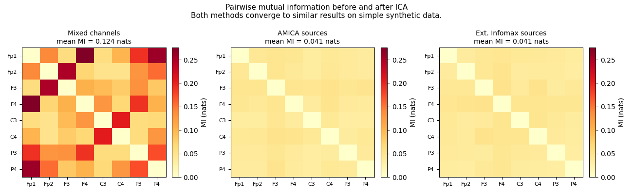
ICA finds components that are as statistically independent as possible. This example demonstrates that property directly: we generate 8 truly independent Laplacian sources, mix them linearly, then show how both AMICA and extended Infomax reduce the pairwise mutual information (MI) between the recovered components compared to the original mixed channels.

A well-fitted decomposition produces a pairwise MI matrix that is close to zero everywhere off the diagonal – each IC is approximately independent of every other. On this clean synthetic dataset both algorithms converge to a similar result. AMICA’s advantage over Infomax becomes more apparent on real EEG data, where source distributions are complex and non-stationary in ways that a fixed sigmoidal nonlinearity cannot capture.

Fitting AMICA ...
AMICA  T=5000  n_orig=8  M=1  J=3
  After sphering: n=8  sldet=-14.7404
  Auto chunk_t=131072 (CPU, ~32 MB L3 target)
  iter     1  lrate=1.000e-01  LL=-3.2987417517  nd=3.212e-01
  Starting Newton at iter 50 ...
  iter   100  lrate=1.000e+00  LL=-3.1859325979  nd=9.877e-04
  iter   200  lrate=1.000e+00  LL=-3.1850218178  nd=5.668e-04
  Done - 200 iterations  final LL=-3.18502182
Fitting extended Infomax ...
/home/runner/work/pyamica/pyamica/examples/plot_mutual_information.py:64: RuntimeWarning: The data has not been high-pass filtered. For good ICA performance, it should be high-pass filtered (e.g., with a 1.0 Hz lower bound) before fitting ICA.
  ica_infomax.fit(raw, picks="eeg")

Mean pairwise MI
  Mixed channels : 0.1243 nats
  AMICA sources  : 0.0413 nats
  Infomax sources: 0.0413 nats

import numpy as np
import matplotlib.pyplot as plt
import mne

from pyamica import AmicaICA, score_mutual_information
from pyamica._mne import _mi_matrix

mne.set_log_level("WARNING")

# ── Synthetic data ─────────────────────────────────────────────────────────────

rng      = np.random.default_rng(42)
N_CH     = 8
T        = 5000
SFREQ    = 250.0
CH_NAMES = ["Fp1", "Fp2", "F3", "F4", "C3", "C4", "P3", "P4"]

# 8 truly independent Laplacian sources, unit variance
S = rng.laplace(0, 1, (N_CH, T))
S = S / S.std(axis=1, keepdims=True)

# Mix with a random matrix
A_true = rng.standard_normal((N_CH, N_CH))
X = A_true @ S
X = X / X.std() * 1e-5          # scale to EEG-like amplitude (~10 µV rms)

info = mne.create_info(CH_NAMES, sfreq=SFREQ, ch_types="eeg")
raw  = mne.io.RawArray(X, info, verbose=False)
raw.set_montage("standard_1020")

# ── Fit AMICA ─────────────────────────────────────────────────────────────────

print("Fitting AMICA ...")
ica_amica = AmicaICA(max_iter=200, verbose=True)
ica_amica.fit(raw, picks="eeg")

# ── Fit extended Infomax ───────────────────────────────────────────────────────

print("Fitting extended Infomax ...")
ica_infomax = mne.preprocessing.ICA(
    n_components=N_CH, method="infomax", random_state=0,
    fit_params=dict(extended=True),
)
ica_infomax.fit(raw, picks="eeg")

# ── Compute MI matrices ────────────────────────────────────────────────────────

mi_mixed   = _mi_matrix(raw.get_data(), n_bins=30)
mi_amica   = score_mutual_information(ica_amica.get_mne_ica(0), raw)
mi_infomax = score_mutual_information(ica_infomax, raw)

idx          = np.triu_indices(N_CH, k=1)
mean_mixed   = mi_mixed[idx].mean()
mean_amica   = mi_amica[idx].mean()
mean_infomax = mi_infomax[idx].mean()

print(f"\nMean pairwise MI")
print(f"  Mixed channels : {mean_mixed:.4f} nats")
print(f"  AMICA sources  : {mean_amica:.4f} nats")
print(f"  Infomax sources: {mean_infomax:.4f} nats")

# ── Plot ───────────────────────────────────────────────────────────────────────

labels = [ch[:3] for ch in CH_NAMES]
vmax   = mi_mixed.max()

fig, axes = plt.subplots(1, 3, figsize=(13, 4))

titles = [
    f"Mixed channels\nmean MI = {mean_mixed:.3f} nats",
    f"AMICA sources\nmean MI = {mean_amica:.3f} nats",
    f"Ext. Infomax sources\nmean MI = {mean_infomax:.3f} nats",
]
matrices = [mi_mixed, mi_amica, mi_infomax]

for ax, mi, title in zip(axes, matrices, titles):
    im = ax.imshow(mi, vmin=0, vmax=vmax, cmap="YlOrRd", aspect="auto")
    ax.set_xticks(range(N_CH))
    ax.set_yticks(range(N_CH))
    ax.set_xticklabels(labels, fontsize=8)
    ax.set_yticklabels(labels, fontsize=8)
    ax.set_title(title, fontsize=10)
    plt.colorbar(im, ax=ax, label="MI (nats)", fraction=0.046, pad=0.04)

fig.suptitle(
    "Pairwise mutual information before and after ICA\n"
    "Both methods converge to similar results on simple synthetic data.",
    fontsize=11,
)
plt.tight_layout()
plt.show()