Basic AMICA Fit

Fit a single-model AMICA (equivalent to Infomax ICA) on synthetic data. Inspects the raw input, convergence via the log-likelihood curve, and confirms that the sphering matrix correctly whitens the data.

import numpy as np
import torch
import matplotlib.pyplot as plt

from pyamica import AMICA

Generate Synthetic Data

Mix 8 independent Laplacian sources with a random matrix.

rng = np.random.default_rng(0)
n_ch, T = 8, 4000

sources = rng.laplace(0, 1, (n_ch, T))
A_true  = rng.standard_normal((n_ch, n_ch))
data    = (A_true @ sources).T.astype("float64")   # (T, n_ch)
X       = torch.from_numpy(data)

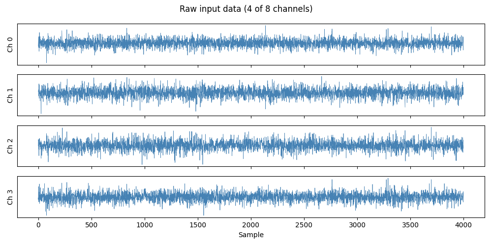
Raw Data

A look at the first 4 channels. Because the sources are Laplacian, the mixture has occasional large spikes.

fig, axes = plt.subplots(4, 1, figsize=(10, 5), sharex=True)
t = np.arange(T)
for i, ax in enumerate(axes):
    ax.plot(t, data[:, i], lw=0.5, color="steelblue")
    ax.set_ylabel(f"Ch {i}")
    ax.set_yticks([])
axes[-1].set_xlabel("Sample")
fig.suptitle("Raw input data (4 of 8 channels)")
fig.tight_layout()
plt.show()

Fit AMICA (M=1)

model = AMICA(n_models=1, max_iter=100, verbose=False)
model.fit(X)

print(f"Iterations:           {model.n_iter_}")
print(f"Final log-likelihood: {model.ll_history()[-1]:.6f}")

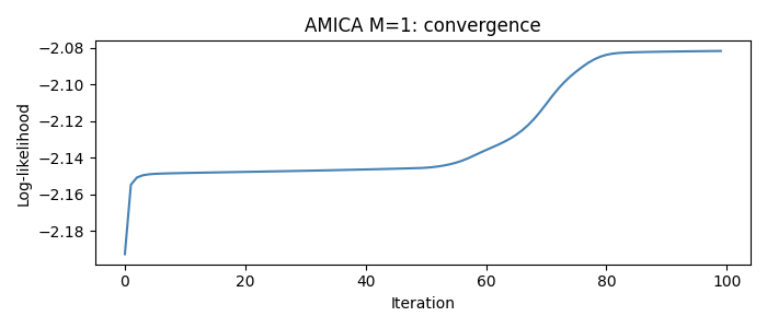
Iterations:           100
Final log-likelihood: -2.081794

Log-Likelihood Curve

The LL should increase monotonically and flatten as the model converges.

fig, ax = plt.subplots(figsize=(7, 3))
ax.plot(model.ll_history().numpy(), color="steelblue")
ax.set_xlabel("Iteration")
ax.set_ylabel("Log-likelihood")
ax.set_title("AMICA M=1: convergence")
fig.tight_layout()
plt.show()

Sphering Matrix

AMICA pre-whitens the data with a ZCA (symmetric) sphering matrix S = V D^{-1/2} V^T (eigendecomposition of the sample covariance).

The defining property of a whitening matrix is that the sphered data has identity covariance: \(S \cdot \text{Cov}(X) \cdot S^T = I\). Verified directly below.

S    = model.sphere_.numpy()              # (n_ch, n_ch)
X_c  = data - data.mean(axis=0)          # centre
Xs   = X_c @ S.T                         # (T, n_ch) - sphered data
cov_sphered = Xs.T @ Xs / T              # should be identity

fig, ax = plt.subplots(figsize=(4, 4))
im = ax.imshow(cov_sphered, vmin=-0.05, vmax=1.05, cmap="RdBu_r")
fig.colorbar(im, ax=ax, shrink=0.8)
ax.set_title("Covariance of sphered data\n(should be identity)")
fig.tight_layout()
plt.show()

residual = np.abs(cov_sphered - np.eye(n_ch)).max()
print(f"Max deviation from identity: {residual:.2e}  (expect < 1e-12)")

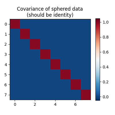
Max deviation from identity: 1.38e-14  (expect < 1e-12)